Predicting Flight Arrival Delays: Machine Learning Approaches
Final Report
Introduction
Air travel, renowned for its speed and global connectivity, remains vulnerable to unforeseen disruptions. Despite the high level of operational planning in the aviation industry, where flight schedules are often determined months in advance, unpredictable variables such as weather, air traffic congestion, and technical issues continue to cause significant delays [1]. These disruptions have wide-ranging economic, environmental, and social impacts. In 2019 alone, flight delays were estimated to cost the U.S. economy approximately $33 billion, encompassing direct airline costs, fuel wastage, crew rescheduling, and indirect effects on connected industries such as hospitality and tourism [8].
Related Work
The prediction of flight delays has attracted research due to its economic, operational, and environmental implications. Traditional statistical models were initially employed to analyze delay causes, however, their limited ability to capture nonlinear interactions between operational, temporal, and meteorological variables has motivated the adoption of machine learning (ML) techniques.
Hatipoğlu and Tosun [1] investigated flight delay prediction at a Turkish airport using multiple ML classifiers, including Logistic Regression, Naïve Bayes, Neural Networks, Random Forest, XGBoost, CatBoost, and LightGBM. Their results demonstrated that ensemble-based approaches, particularly XGBoost, achieved superior predictive performance, reaching an accuracy of 80%. The study also addressed class imbalance using the Synthetic Minority Over-Sampling Technique (SMOTE) and applied SHAP (SHapley Additive exPlanations) for model interpretability, revealing the relative contribution of operational and weather-related features.
Similarly, Meel et al. [3] and R. G. et al. [9] evaluated multiple ML classifiers such as Logistic Regression, Decision Trees, Bayesian Ridge, Random Forest, Gradient Boosting, and Support Vector Machines for flight delay prediction. Their results confirmed that tree ensemble models and kernel methods outperform simpler regression baselines by effectively capturing complex dependencies in flight operations, weather, and air traffic congestion. The model proposed by R. G. et al. [9] achieved an accuracy of 95%, highlighting the scalability of ML-driven approaches when trained on large, heterogeneous datasets.
Li et al. [4] extended this line of research using data from the U.S. Bureau of Transportation Statistics (BTS) to compare several ML and computational intelligence methods, including linear regression, random forest, gradient boosting, Gaussian regression, and genetic programming, for predicting arrival delay time. Their findings indicated that genetic programming provided the best predictive accuracy, emphasizing the benefit of evolutionary optimization methods in modeling aviation delays.
Finally, Huynh et al. [5] conducted a systematic review of flight delay forecasting models, concluding that Artificial Neural Networks (ANNs) and Random Forests are the most robust and widely used frameworks. The review further emphasized the importance of feature selection, identifying flight attributes, meteorological conditions, and temporal factors as critical inputs that significantly influence model performance.
Collectively, prior studies demonstrate that machine learning offers a powerful framework for delay prediction by integrating operational, temporal, and environmental variables. However, most existing works are either restricted to specific regions or employ older datasets. Moreover, while ensemble methods and neural networks consistently deliver high predictive accuracy, model generalization across airports and varying traffic conditions remains an open challenge. This motivates our study, which focuses on developing and evaluating ML-based classifiers to predict arrival delays at Hartsfield–Jackson Atlanta International Airport (ATL) using recent BTS data spanning 2019–2025, thereby contributing a large-scale and region-specific analysis to the growing body of literature on flight delay forecasting.
Dataset
For this project, we use flight performance data from the U.S. Bureau of Transportation Statistics (BTS),
specifically arrivals at Hartsfield–Jackson Atlanta International Airport (ATL) from 11 different airlines.
The dataset covers domestic flights over the past five years (2019-2025, excluding 2020 and 2021 due to COVID-19 disruptions).
It contains detailed records such as scheduled and actual times, delay, cause of delay, etc.
Dataset link: BTS On-Time Arrival Data [6].
Problem Definition
According to the Bureau of Transportation Statistics (BTS), in 2024 there were 787,630 arrival delays across the United States [7], underscoring the scope and recurrence of this issue. Machine learning has been used for several years as a tool to address this issue, and it has been proven to be a powerful and effective one. To standardize our analysis, we adopt the Federal Aviation Administration (FAA) definition of a delay, which considers a flight delayed if its arrival time is more than 15 minutes later than scheduled. This definition provides a consistent framework for modeling and evaluating flight delays.
In this project, we formulate the prediction task primarily as a binary classification problem, where the goal is to determine whether a flight will arrive on time or delayed based on pre-departure features. Additionally, we also formulate the task as a regression problem that predicts the expected delay duration (in minutes) for flights identified as delayed. Together, these complementary approaches enable both categorical delay detection and quantitative delay estimation, offering a more comprehensive view of flight delay behavior and potential mitigation strategies.
Methods
For our project on predicting flight delays, we will use a mix of preprocessing steps and supervised machine learning models. The goal is to clean and prepare the data so that our models can make reliable predictions.
Data Preprocessing
Before implementing the model, we implemented an extensive preprocessing pipeline to ensure the data remained consistent and reliable for all models.
The preprocessing procedures was executed in the notebooks 01_exploratory_data_analysis.ipynb, 02_data_preprocessing.ipynb, 03_feature_engineering.ipynb
with the help of scripts under the directory src/data/.
Exploratory Data Analysis
The dataset from the Bureau of Transportation Statistics (BTS)
[6] includes flights from
11 major U.S. airlines spanning 2019–2025 (until July 31).
Separate .csv files for each carrier and year were merged into a unified dataset (.csv File).
While doing exploratory data analysis (EDA), we analysed the distributions of the features and also summary of the statistics of the features.
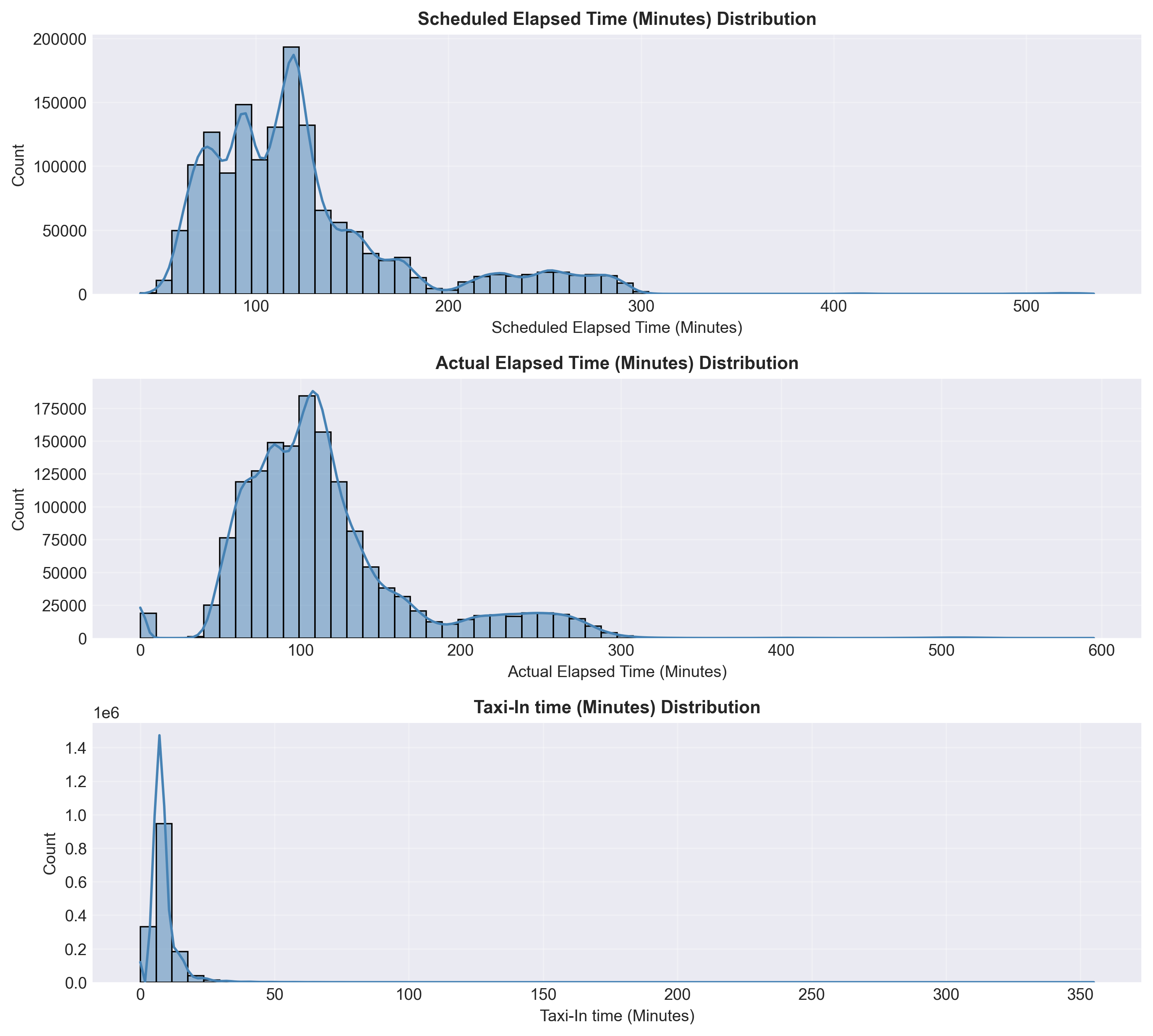
It can be seen in Figure 1a and Figure 1b that expected flight durations were 60–200 minutes and there were highly right-skewed delay variables.
Most flights arrived on time, while a small subset experienced long carrier- or aircraft-related delays.
These insights guided data cleaning, outlier handling, and the creation of the binary label (Delay or Not Delayed).
The correlation matrix (Figure 2) shows strong relationships between Scheduled and Actual Elapsed Times (r ≈ 0.94), confirming internal data consistency. Arrival Delay correlates most strongly with Carrier Delay (r ≈ 0.75) and Late Aircraft Arrival (r ≈ 0.52), indicating that operational and turnaround factors are the primary drivers of delay propagation. Other causes such as Weather and Security exhibit weaker correlations, reflecting their infrequent nature.
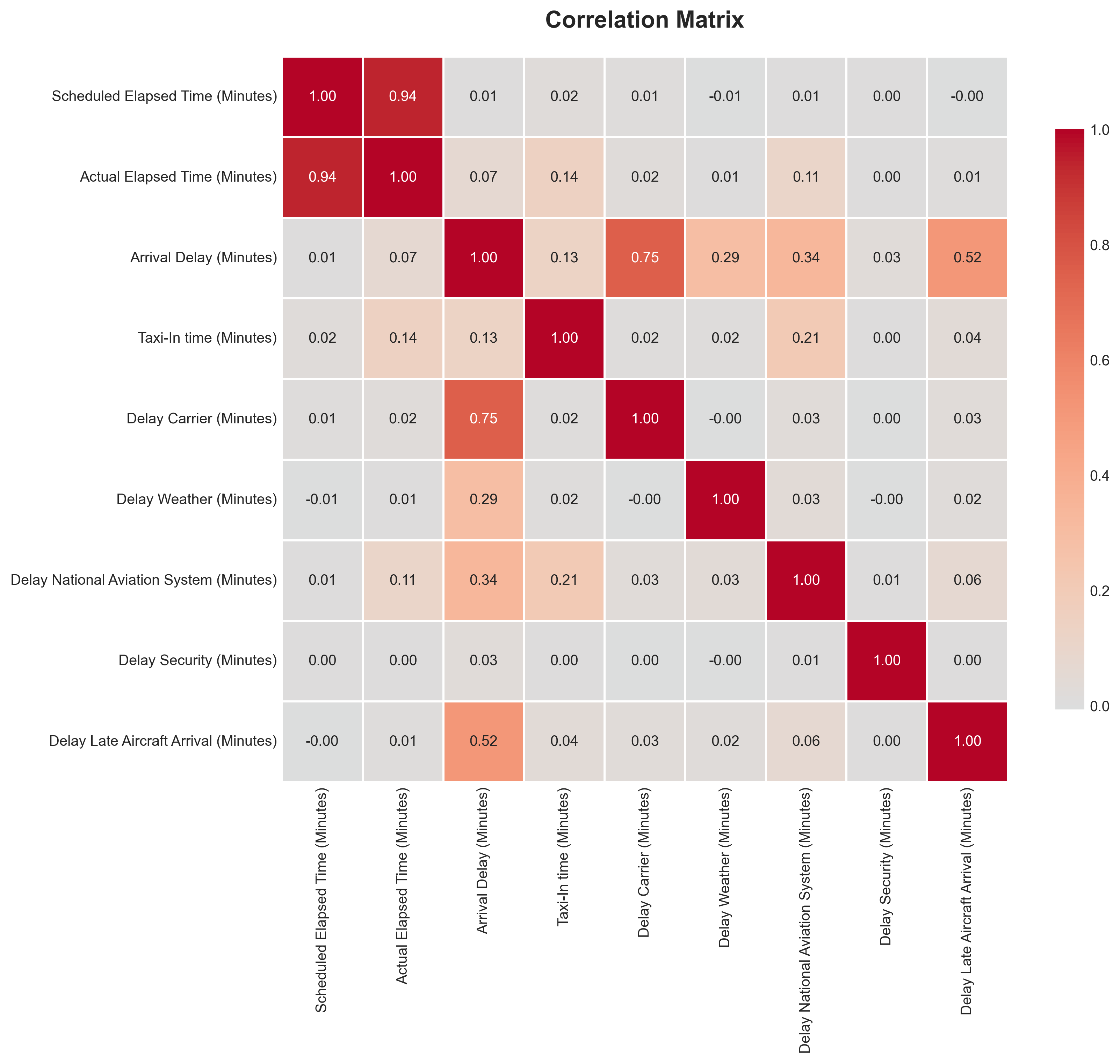
Overall, EDA confirmed the dataset’s consistency and revealed that delay patterns are primarily caused by carrier and aircraft factors. These findings provided the foundation for next steps.
Data Cleaning and Transformation
After data integration, a systematic preprocessing pipeline was applied to ensure data quality and consistency.
Invalid rows were removed, data types were standardized, and categorical variables were converted to appropriate formats.
Invalid rows with missing critical information such as flight times or delay components were removed to ensure record completeness.
Data types were standardized by converting date fields to datetime format, ensuring numerical columns (e.g., elapsed and delay times)
used consistent integer types, and coercing non-numeric values to NaN where necessary.
Categorical variables, including Carrier Code and Origin Airport, were converted to efficient
category types to improve memory usage and facilitate encoding during modeling.
Missing numeric values were imputed using the median, while categorical gaps such as Tail Number were filled with Unknown.
Outliers were reviewed but retained to preserve the natural variability of flight operations, as the selected models are robust to such values.
Duplicates were eliminated, and date fields were normalized to the canonical format Date (YYYY-MM-DD).
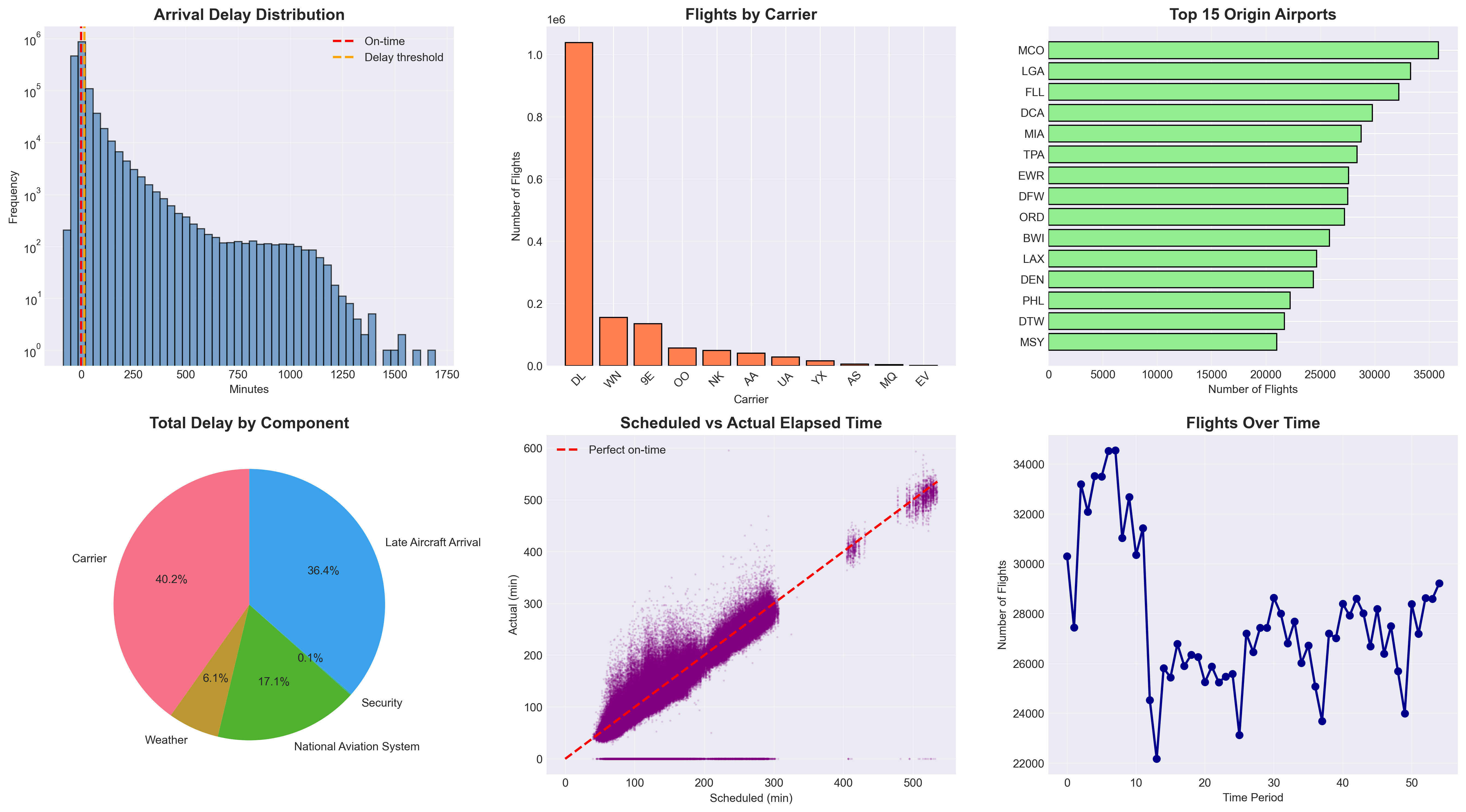
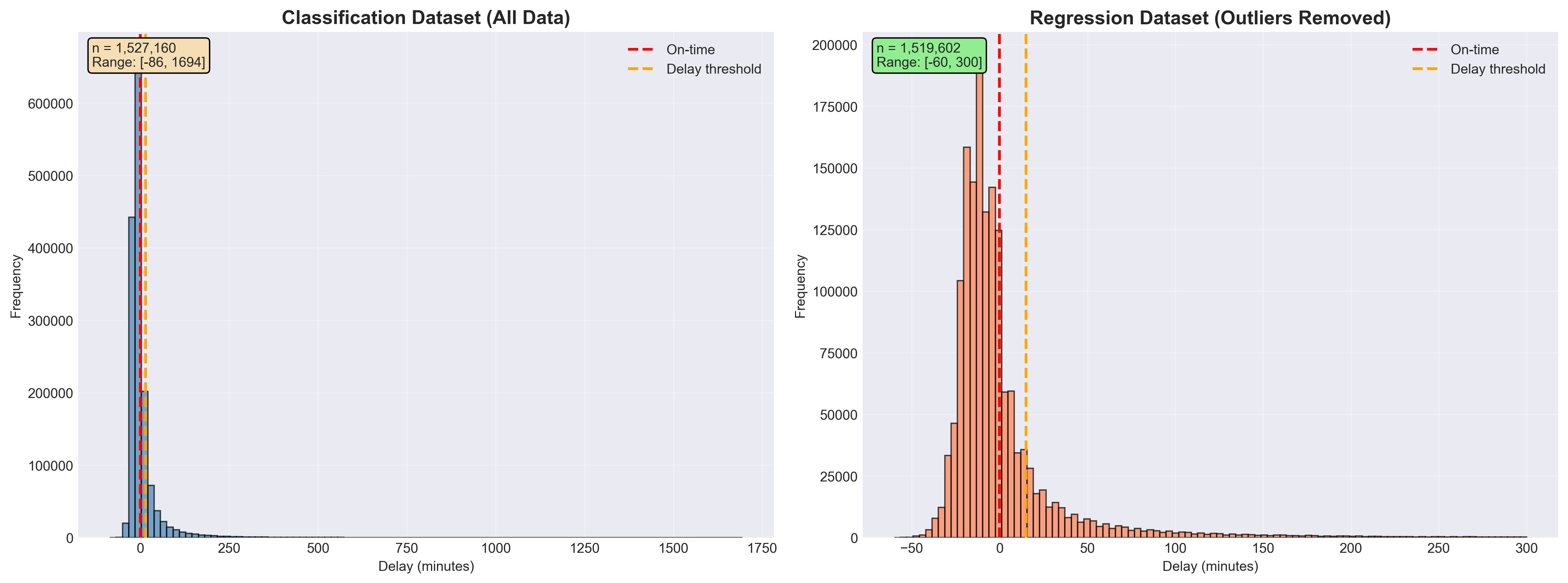
Figure 3 summarizes the dataset after preprocessing. The cleaned data exhibit consistent structure and realistic operational patterns: most flights last between 60–200 minutes, carrier-related delays dominate total delay composition, and the strong correspondence between scheduled and actual elapsed times confirms internal data reliability.
Feature Engineering
Building on the cleaned dataset, new features were engineered to capture temporal, categorical, and operational factors influencing flight delays.
Binary indicators such as IsWeekend and Is_Holiday_Period were derived from flight dates to represent temporal travel patterns,
while Season was encoded into four categories (Fall, Spring, Summer, Winter) to capture seasonal variation.
The target variable Is_Delayed was defined according to the FAA’s 15-minute threshold.
Categorical variables were transformed for modeling: Carrier Code was one-hot encoded,
Origin Airport was label-encoded, and Season was numerically encoded for model compatibility.
The final engineered dataset included 16 predictive features spanning operational, temporal, and categorical dimensions:
- Operational:
Scheduled Elapsed Time (Minutes),IsWeekend,Is_Holiday_Period - Carrier-specific dummies (11):
Carrier_9E,Carrier_AA,Carrier_AS,Carrier_DL,Carrier_EV,Carrier_MQ,Carrier_NK,Carrier_OO,Carrier_UA,Carrier_WN,Carrier_YX - Encoded categorical:
Origin_Airport_Encoded,Season_Encoded
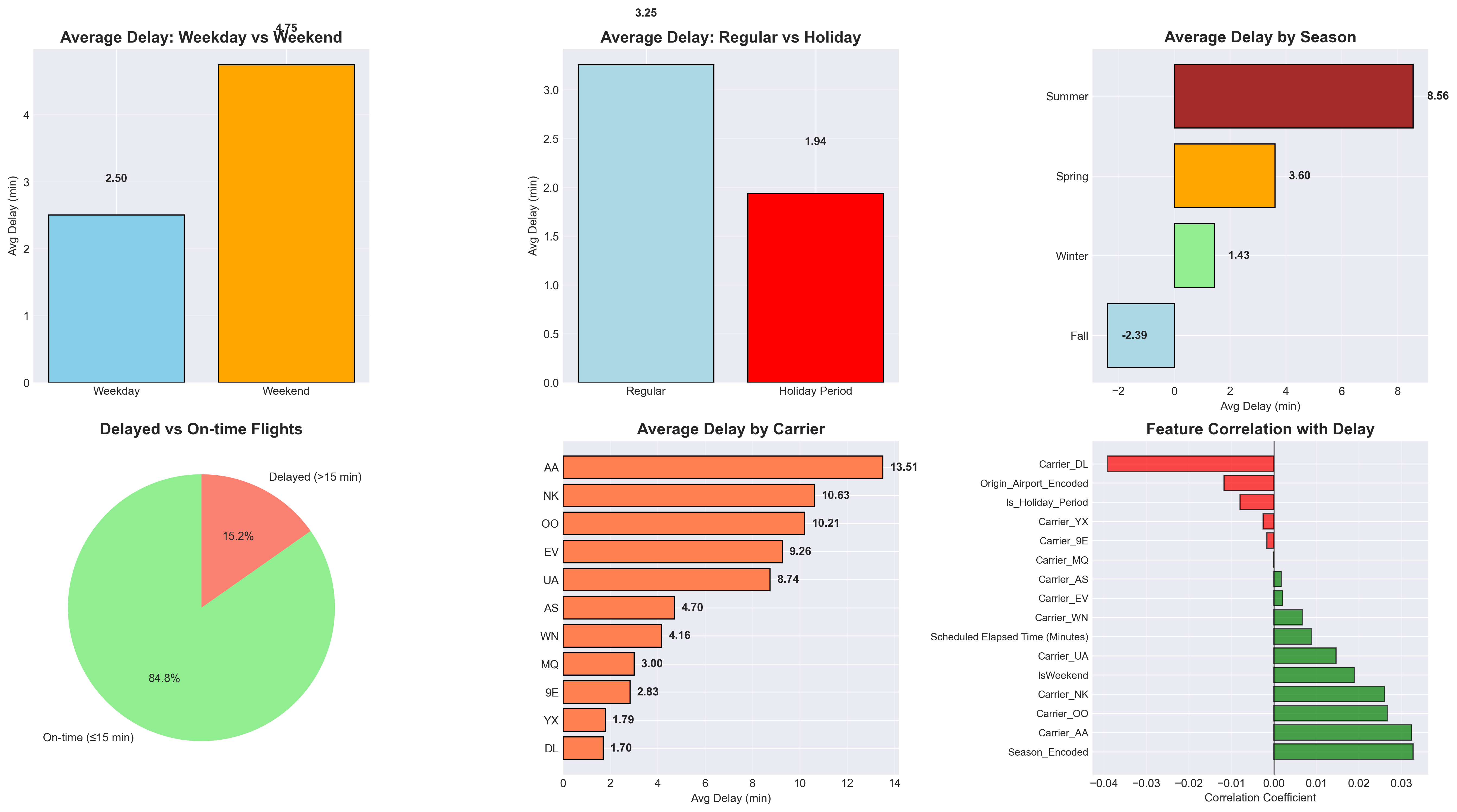
Figure 4 visualizes these engineered features and their relationships. Delays tend to be slightly higher during weekends and summer months, while carrier-level patterns highlight differences in operational performance. Together, these features provide a compact yet comprehensive representation of factors relevant to flight delay prediction.
Feature Engineering for Regression
For the regression task, the feature engineering process remained largely identical to that used for classification,
with one key difference: instead of the binary target variable Is_Delayed, we used
Arrival Delay (Minutes) from the original dataset as the continuous target.
To improve model robustness and prevent extreme outliers from skewing predictions, we implemented
adjustable range filtering with default thresholds of min = -60 minutes and
max = 300 minutes. This approach removed flights with unrealistic early arrivals
(more than 60 minutes ahead of schedule) and extremely long delays (exceeding 5 hours),
while preserving the natural variability of operational delays within reasonable bounds.
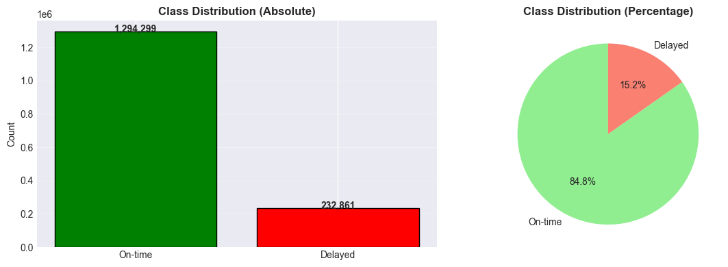
Class Distribution
The class distribution shown in Figure 6 reveals a significant imbalance: approximately 84.8 % of flights arrived on time, while only 15.2 % were delayed. This skew can bias models toward predicting the majority “on-time” class, resulting in poor sensitivity to delay events. To address this, we evaluated both imbalanced (default) and balanced model variants in subsequent experiments. As discussed in class, ensemble methods such as Random Forests often perform reasonably well even under class imbalance, but applying explicit class weighting can further improve the detection of minority-class instances.
Machine Learning Models
Logistic Regression
We adopted a phased project strategy, beginning binary classification before advancing to regression.
This allows us to tackle a simpler task and evaluate the initial model's performance to validate the quality of our dataset and our data preprocessing techniques before investing time in more complex regression models.
Logistic Regression, which was the first supervised learning algorithm introduced in class, was selected as our first (baseline) model due to its simplicity, computational speed, and also interpretability. The algorithm estimates the probability that a given instance belongs to the “delayed” class. As a linear classifier, it provides coefficients that quantify the influence of each feature on the likelihood of a flight delay. This property not only facilitates a transparent understanding of model behavior but also allows domain experts, such as airline and airport operations personnel, to validate the model’s reasoning and potentially integrate its predictions into operational decision-making processes. Therefore, this model could have a direct real-world impact in optimizing air traffic logistics.
We performed 3-Fold Cross-Validation, meaning the dataset was divided into three equally sized folds while preserving the class distribution in each split. In each iteration, it is trained on two folds and validated on the remaining one. This enables us to select the best value for the regularization hyperparameter λ (lambda), which mitigates the risk of overfitting to any subset of the data. We are currently using 0.5 as the probability threshold for classification.
Random Forest Classifier
After establishing the baseline with Logistic Regression, we implemented a Random Forest Classifier to capture nonlinear dependencies that a linear model cannot represent. Random Forests are ensemble methods that construct multiple decision trees on random subsets of data and features, then aggregate their outputs through majority voting and it was mentioned in the lecture, that ensemble methods handle imbalanced data well.
We began by training a baseline Random Forest using default parameters, followed by two improved variants:
a balanced model addressing class imbalance via class_weight='balanced',
and a tuned model optimized using RandomizedSearchCV
with F1-score as the objective metric.
The tuning process explored the number of estimators, tree depth, and minimum sample thresholds
(n_estimators from [100, 200, 300];
max_depth from [10, 20, 30, None];
min_samples_split from [2, 5, 10, 20];
min_samples_leaf from [1, 2, 4, 10]).
Three-fold cross-validation was used to ensure stable generalization across data splits, similarly to the approach used in logistic regression.
The resulting tuned model demonstrated an improved balance between recall and precision compared to the baseline, indicating its effectiveness in identifying delayed flights while limiting false positives. This makes Random Forest a practical choice for early delay detection systems where minimizing missed delay alerts is more critical than achieving perfect precision.
Random Forest Regressor
To extend our analysis beyond binary delay prediction, we employed a Random Forest Regressor to directly model the magnitude of arrival delay in minutes. Whereas classification captures whether a flight is delayed, regression provides more operationally useful estimates of how much delay to expect. Random Forests are particularly well-suited for this task due to their ability to model nonlinear interactions, handle heterogeneous features, and remain robust to outliers in delay values an important property given the heavy-tailed nature of real-world delay distributions.
We first trained a baseline Random Forest using default settings, then developed an optimized model using RandomizedSearchCV with RMSE, MAE, and R² as the evaluation metrics. Because training full forests on the entire dataset was computationally expensive, we performed hyperparameter search using a subsampled version of the training data. The search explored key structural parameters including the number of trees, tree depth, and minimum node sizes:
n_estimators from {150, 250, 400},
max_depth from {None, 15, 25, 35},
min_samples_split from {2, 5, 10},
min_samples_leaf from {1, 2, 4, 8},
max_features = "sqrt", bootstrap = True.
The randomized search performed k-fold cross-validation to ensure stability across data splits,
while limiting the total number of configurations via n_iter to keep computation feasible.
After tuning, the best-performing model was:
RandomForestRegressor( n_estimators=400, max_depth=15, max_features="sqrt", min_samples_leaf=8, n_jobs=-1, random_state=42 )
The Random Forest Classifier and Regressor algorithm was selected because of its ability to model complex relationships, handle mixed feature types, and remain robust to outliers and noise. Unlike linear models, it can naturally capture interactions between operational and temporal variables, such as how flight duration, departure airport, and seasonal patterns jointly influence delay probability. Additionally, its feature importance output provides interpretability by quantifying each variable's contribution to the prediction, making it suitable for both predictive and diagnostic insights. The results will be discussed in the next section. Futhermore, Mahdi mentioned that ensemble algorithms work best with imbalanced data, hence a consideration for the choice.
Multi-Layer Perceptron Classifier
In addition to the linear (Logistic Regression) and tree-based (Random Forest) models, we implemented a
Multi-Layer Perceptron (MLP) Classifier to capture higher-order, nonlinear relationships
between the engineered features and the binary delay label Is_Delayed. While Logistic Regression
provides a strong interpretable baseline and Random Forests handle feature interactions via ensembles of trees,
an MLP offers a complementary inductive bias as a universal function approximator. This allows the model to
learn smooth, multi-dimensional decision boundaries that may better reflect complex interactions between
carrier, origin airport, seasonality, and operational factors.
Because gradient-based neural networks are highly sensitive to feature scaling, we first standardized all
input features using StandardScaler, fitting the scaler on the training set only and applying
the same transformation to the test set. Each feature was transformed to have zero mean and unit variance,
ensuring that all dimensions contribute comparably to the optimization process and preventing features with
large numerical ranges from dominating the gradients.
For the classification task, the MLP receives a feature vector
x ∈ ℝd (with d = 16 engineered features) and outputs the probability that a
flight is delayed. The network architecture can be summarized as:
- Input layer with 16 neurons (one per engineered feature).
-
Two fully connected hidden layers with
(100, 50)neurons in the baseline configuration. -
Hidden activation: ReLU or
tanh(selected via grid search), providing nonlinearity and enabling the network to model complex decision surfaces. -
Output layer: single neuron with logistic / sigmoid output, representing
P(Is_Delayed = 1 | x).
We trained the MLP Classifier using the Adam optimizer, which adapts learning rates per parameter and typically converges faster than vanilla stochastic gradient descent. The main hyperparameters for the baseline model were:
hidden_layer_sizes = (50, )activation = "relu"solver = "adam"alpha = 1e-3(L2 regularization strength)learning_rate = "constant"learning_rate_init = 1e-3max_iter = 200random_state = 42
To address the pronounced class imbalance (≈ 15% delayed, 85% on time), we used
class-balanced sample weights during training. Specifically, we computed per-sample weights
with class_weight = "balanced", which scales the loss contribution of each class inversely to
its frequency. As a result, misclassifying delayed flights incurs a higher penalty than misclassifying
on-time flights, encouraging the network to pay more attention to the minority delay class.
To improve generalization and reduce training time, we optionally enabled
early stopping. In this setting, the MLP reserves 10% of the training data as an internal
validation set (validation_fraction = 0.1) and stops training if the validation score does not
improve for 10 consecutive epochs (n_iter_no_change = 10). This prevents overfitting to the
training set and automatically selects an appropriate number of training iterations.
Finally, we performed hyperparameter tuning using GridSearchCV with
3-fold cross-validation and F1-score as the optimization metric, reflecting our
focus on balancing precision and recall for the delayed class. The grid explored:
hidden_layer_sizes ∈ {(50,), (100,), (100, 50), (100, 50, 25)}activation ∈ {"relu", "tanh"}alpha ∈ {1e-4, 1e-3, 1e-2}learning_rate_init ∈ {1e-3, 1e-2}
During tuning we set max_iter = 300 with early_stopping = True to keep the search
computationally feasible. The tuned network has 2 hidden layers (100, 50), uses relu as the activation function, has a regularization strength of 0.001 and a learning rate of 0.01.
Multi-Layer Perceptron Regressor
For the regression task, we used a Multi-Layer Perceptron Regressor with an architecture
closely mirroring the classifier, but trained to predict a continuous target:
Arrival Delay (Minutes). As described in the preprocessing section, we restricted the delay
range to [−60, 300] minutes to remove extreme outliers and ensure a more stable regression target, while
retaining the natural variability of operational delays.
As with the classifier, all input features were standardized using StandardScaler fitted on the
training data. The regressor operates on the same engineered feature space (16 features) and has the
following architecture:
- Input layer with 16 neurons.
- Two or three fully connected hidden layers with 50–100 neurons each, depending on the configuration (baseline vs. tuned).
-
Hidden activation: ReLU in the baseline model, with
tanhadditionally considered during hyperparameter tuning. - Output layer: single linear neuron predicting the delay in minutes, optimized using mean squared error (MSE) loss.
The baseline MLP Regressor used the same training configuration as the classifier:
hidden_layer_sizes = (50, )activation = "relu"solver = "adam"alpha = 1e-3learning_rate_init = 1e-3,learning_rate = "constant"max_iter = 150,random_state = 42
As with the classifier, we employed early stopping with a 10% validation split and a patience of 10 epochs to prevent overfitting and to automatically determine an appropriate stopping point. Training time and convergence behavior were monitored via the optimization loss printed at each iteration, allowing us to verify that the network reached a stable minimum without diverging.
To systematically explore the design space and avoid manually guessing hyperparameters, we performed grid search hyperparameter tuning with 3-fold cross-validation. The search space was identical in structure to the classifier grid but used regression-oriented scoring:
hidden_layer_sizes ∈ {(50,), (100,), (100, 50), (100, 50, 25)}activation ∈ {"relu", "tanh"}alpha ∈ {1e-4, 1e-3, 1e-2}learning_rate_init ∈ {1e-3, 1e-2}- Scoring metric: negative mean squared error (minimizing RMSE).
During tuning, we again set max_iter = 300 and enabled early_stopping = True to keep
the search efficient. The best-performing configuration selected by GridSearchCV used a network
with two hidden layers (50, 25) , nonlinear tanh activations, and a slightly stronger
L2 penalty (0.01) than the baseline.
XGBoost (Gradient Boosting)
To complement the tree ensemble and neural network approaches, we implemented XGBoost (Extreme Gradient Boosting) for both classification and regression tasks. XGBoost is a highly efficient gradient boosting framework that builds an ensemble of decision trees sequentially, where each tree corrects the errors of its predecessors. Unlike Random Forests, which grow trees independently, XGBoost uses gradient descent optimization to minimize a differentiable loss function, making it particularly effective for structured/tabular data.
For the regression task, we trained an XGBRegressor to predict
Arrival Delay (Minutes), while for classification, we used an
XGBClassifier to predict the binary Is_Delayed label.
Both models were initialized with baseline hyperparameters:
n_estimators = 100(number of boosting rounds)max_depth = 3(maximum tree depth)learning_rate = 0.1(shrinkage parameter)random_state = 42
To optimize performance, we performed Randomized Search with 3-fold Cross-Validation over the following hyperparameter distributions:
n_estimators ∈ [500, 2000]max_depth ∈ [3, 10](regression) /[3, 8](classification)learning_rate ∈ [0.01, 0.3]subsample ∈ [0.6, 1.0](row sampling ratio)colsample_bytree ∈ [0.6, 1.0](column sampling ratio)scale_pos_weight ∈ [1, 5](classification only, to handle class imbalance)
For regression, we optimized using negative mean absolute error (MAE) as the scoring metric,
while for classification, we used F1-score to balance precision and recall.
The search performed 25 iterations with n_jobs=-1 for parallel processing,
and selected the best configuration based on cross-validated performance.
XGBoost was chosen for its ability to handle imbalanced datasets, capture complex nonlinear relationships,
and provide regularization through parameters like max_depth and learning_rate.
Its sequential boosting strategy allows it to focus on correcting residual errors, sometimes yielding
superior performance compared to independently trained models like Random Forests.
Results and Discussion
To better understand model performance, we analyzed the confusion matrices for both the unbalanced and balanced logistic regression and random forest models.
Logistic Regression
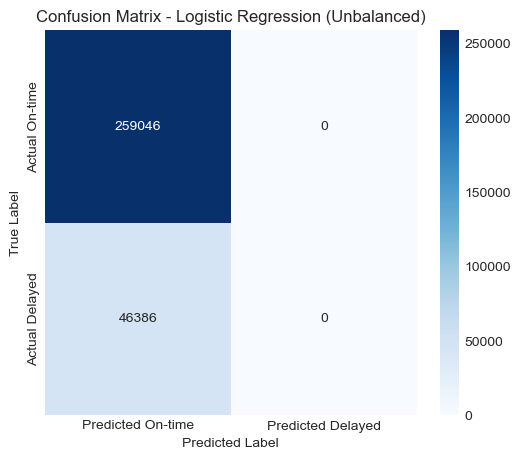
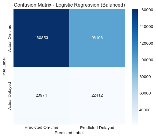
The unbalanced model predicted almost all flights as “not delayed,” resulting in a confusion matrix heavily skewed toward the majority class. The balanced model showed a more reasonable distribution of predictions, correctly identifying a portion of the delayed flights, although it also misclassified a significant number of non-delayed flights as delayed.
These visualizations highlight the impact of class imbalance and the importance of accounting for it when modeling delay prediction problems.
Visualizations
Confusion Matrix — Unbalanced
Confusion Matrix — Balanced
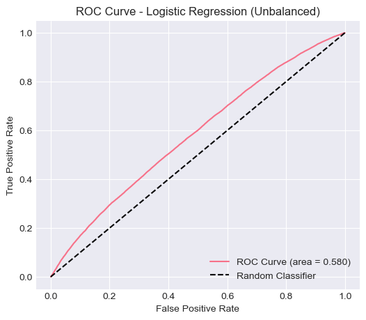
ROC Curve — Unbalanced
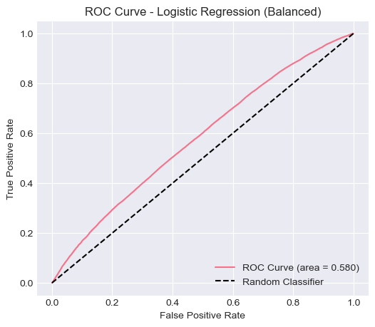
ROC Curve — Balanced
Quantitative Metrics
| Model | Accuracy | Precision | Recall | F1-Score | ROC-AUC |
|---|---|---|---|---|---|
| Logistic Regression (Unbalanced) | 0.8481 | 0.0000 | 0.0000 | 0.0000 | 0.5805 |
| Logistic Regression (Balanced) | 0.6000 | 0.1858 | 0.4832 | 0.2684 | 0.5805 |
The unbalanced model achieved high accuracy (0.8481) but failed to identify any delayed flights (recall = 0), indicating that it learned to always predict the majority class. This is a common issue in imbalanced datasets, where accuracy can be misleading because predicting the dominant class yields superficially strong results.
When class weights were balanced, the model’s recall improved to 0.4832, and F1-score increased to 0.2684, showing that the model was able to capture more delayed flights, albeit with lower overall accuracy. The ROC-AUC (0.5805) remained roughly the same in both cases, suggesting that the model’s overall discriminative ability between delayed and non-delayed flights remains limited.
Analysis of the Logistic Regression Model
The logistic regression model serves as a strong baseline for this classification problem. Its interpretability and computational efficiency make it suitable for early-stage analysis. However, the results indicate that the model struggles with the class imbalance inherent in the dataset, where only 15% of flights are delayed.
In the unbalanced case, the model simply defaulted to predicting the majority class (no delay), leading to poor performance on minority cases. Applying balanced class weights improved detection of delayed flights, but the model still lacked predictive strength. This suggests that the linear decision boundary of logistic regression may not adequately capture the complex, nonlinear patterns associated with flight delays (e.g., interactions between weather, airport congestion, and time of day).
Feature Importance Analysis
The logistic regression model also allows us to interpret which variables most strongly influence flight delay predictions.
The top 15 most influential features (by absolute coefficient value) indicate that seasonality (Season_Encoded) has the strongest positive association with delays, suggesting that certain times of the year (e.g., winter or summer travel peaks) are more prone to delays.
Several airline carrier indicators (e.g., Carrier_DL, Carrier_NK, Carrier_AA) also show substantial influence, reflecting performance differences among airlines.
Operational features such as Scheduled Elapsed Time (Minutes) and IsWeekend further contribute, implying that longer scheduled flights and weekend departures have a higher likelihood of delay.
In contrast, some features like Origin_Airport_Encoded or Is_Holiday_Period show negative or weaker coefficients, indicating they are less predictive or associated with fewer delays in this dataset.
Overall, this analysis highlights that both temporal factors (season, weekend) and carrier-specific effects play a key role in determining whether a flight is delayed.
Random Forest Classifier
The Random Forest classifier was trained under two configurations, the original (imbalanced), and tuned model (balanced). The confusion matrices and ROC curves below compare the model’s ability to correctly identify delayed flights before and after applying class weighting and hyperparameter tuning. The tuned model shows improved recall, and F1-score for the delayed class while maintaining a similar overall ROC–AUC, indicating better sensitivity to minority cases without overfitting.
Visualizations
Confusion Matrix — Original
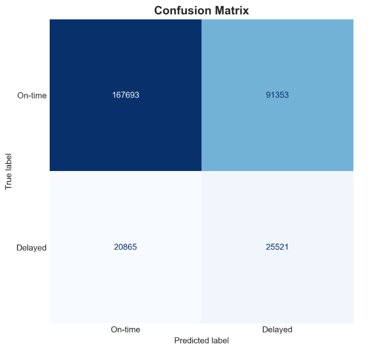
Confusion Matrix — Balanced (Tuned)
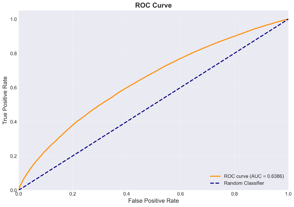
ROC Curve — Original
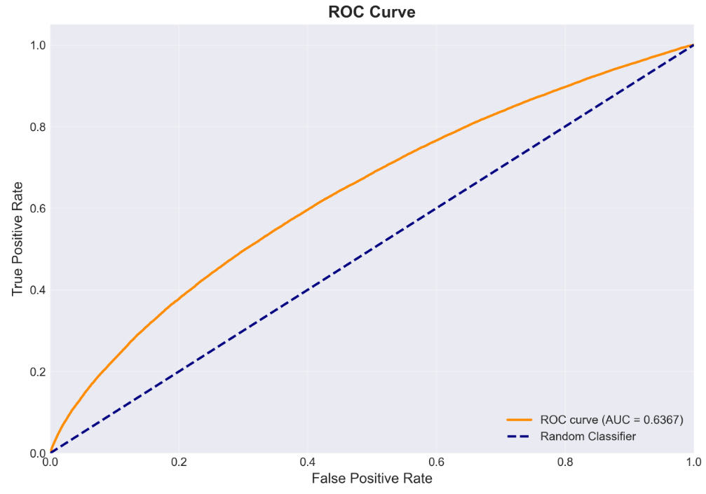
ROC Curve — Balanced (Tuned)
Quantitative Metrics
| Model | Accuracy | Precision | Recall | F1-Score | ROC-AUC |
|---|---|---|---|---|---|
| Random Forest (Original) | 0.8480 | 0.4623 | 0.0071 | 0.0141 | 0.6386 |
| Random Forest (Balanced) | 0.6326 | 0.2184 | 0.5502 | 0.3126 | 0.6367 |
Quantitatively, the balanced model improved recall (approximately 0.55) compared to the original model’s near-zero recall (0.007), confirming that class weighting allowed the model to recognize more delay cases. While overall accuracy decreased (0.63 from 0.85), this trade-off is expected and desirable for imbalanced data. The ROC–AUC remained stable at around 0.64, suggesting the model's ability to discriminate between on-time and delayed flights improved in balance rather than separability.
Analysis of Random Forest Classifier
The tuned Random Forest used n_estimators = 200, max_depth = 20,
min_samples_split = 20, min_samples_leaf = 4, and
class_weight = 'balanced'. This configuration achieved the highest F1-score (≈0.31)
and a stable ROC–AUC (≈0.64). Feature importance analysis revealed that
Scheduled Elapsed Time, Origin Airport, and Season were the most influential predictors,
together accounting for over 80% of the model’s decision weight.
This indicates that both operational and temporal factors strongly shape delay likelihood, while
individual carriers contribute comparatively less.
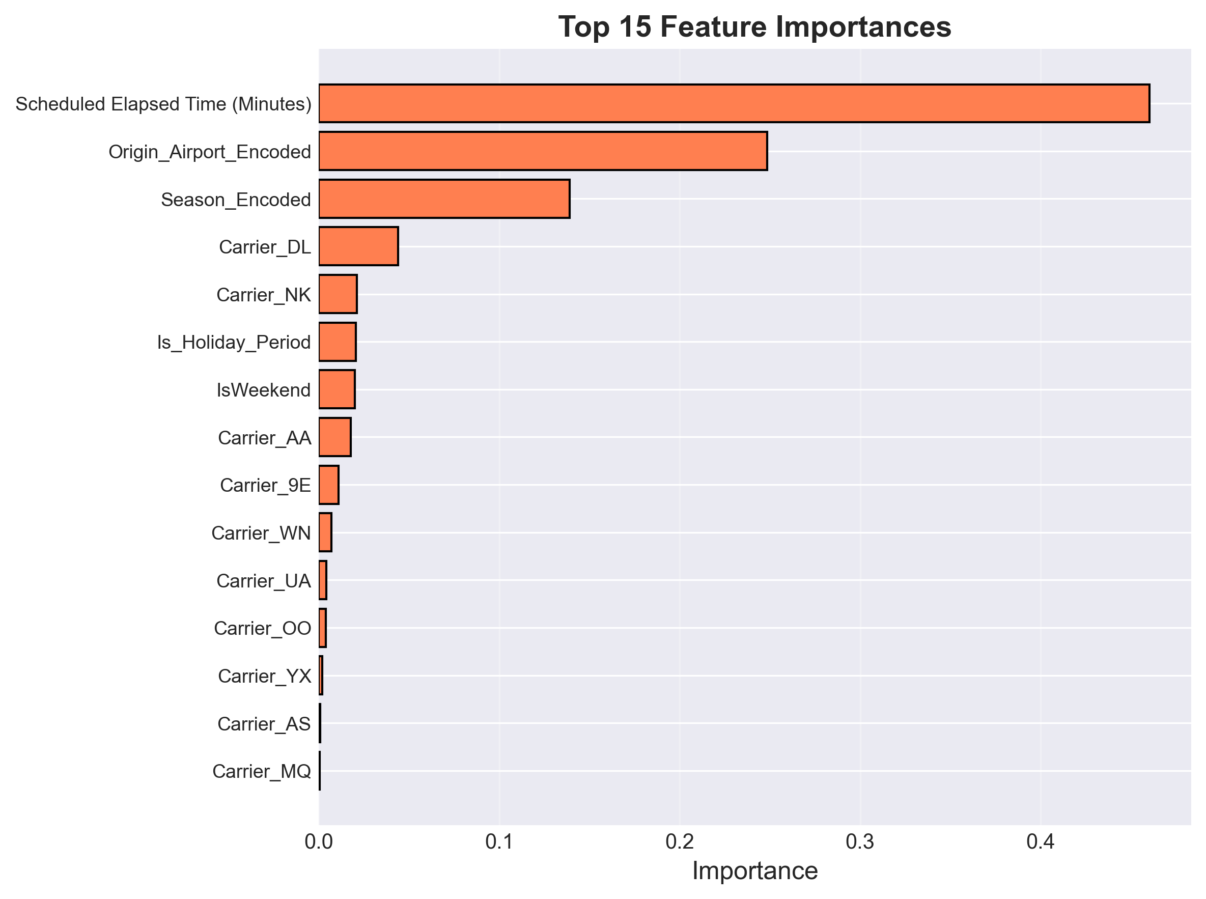
Top 15 Feature Importances — Random Forest model highlighting operational and temporal predictors.
Overall, the Random Forest model demonstrates robustness to noise and outliers and benefits from class weighting to improve minority detection. Its moderate discriminative power suggests that further improvement may depend on integrating external variables such as weather, air traffic congestion, and time-of-day effects to capture real-world variability in flight delays.
Random Forest Regressor
The Random Forest Regressor was evaluated to estimate the magnitude of arrival delay (in minutes), providing a finer-grained perspective than binary delay prediction. The model was trained using the tuned configuration identified through a randomized hyperparameter search, and its performance was assessed using RMSE, MAE, and R². The results and visualizations below summarize the model’s predictive behavior and its limitations when applied to real-world flight delay regression.
Visualizations
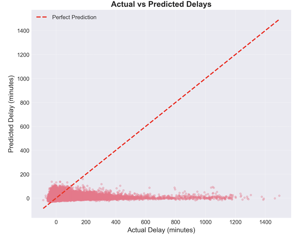
Actual vs Predicted Delay — Predictions cluster near zero, showing underestimation of large delays.
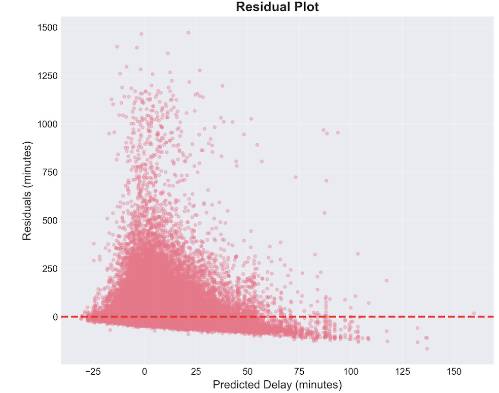
Residual Plot — High variance and increasing positive residuals for larger predicted delays.
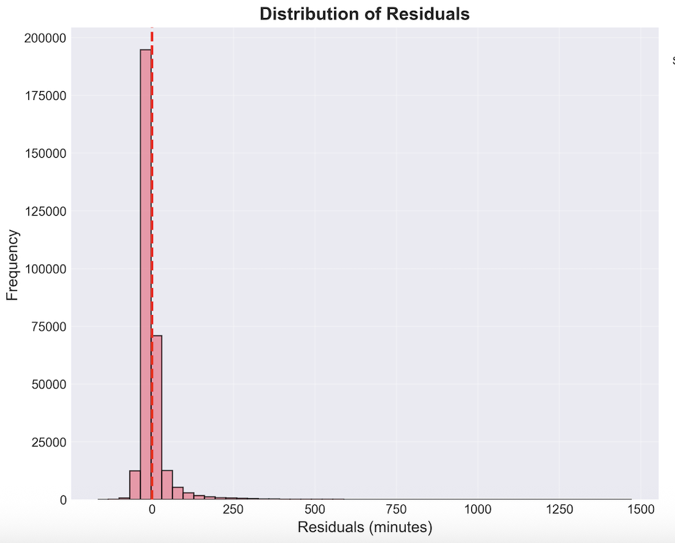
Distribution of Residuals — Strong right skew reflecting heavy-tailed delay behavior.
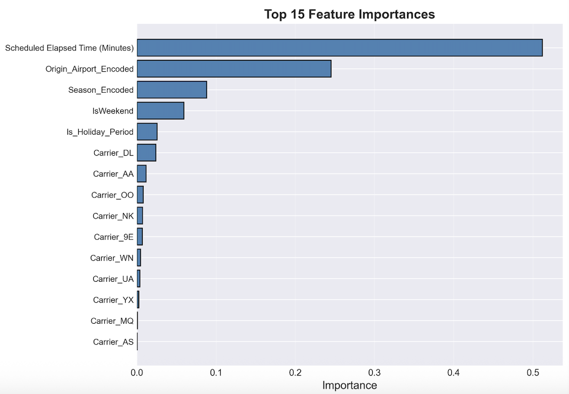
Top 15 Feature Importances — Scheduled Elapsed Time dominates the regressor’s decisions.
Quantitative Metrics
| Dataset | RMSE (minutes) | MAE (minutes) | R² |
|---|---|---|---|
| Training Set | 33.8380 | 19.2958 | 0.0515 |
| Test Set | 34.1714 | 19.5276 | 0.0360 |
Analysis of Random Forest Regressor
Across both training and test sets, the Random Forest Regressor achieved an RMSE of approximately 34 minutes and an MAE of roughly 19.5 minutes. These values are consistent across splits, indicating that the model does not overfit; however, the low R² (≈0.03) suggests that the model explains only a small portion of the variance in arrival delays.
The Actual vs. Predicted plot shows a pronounced clustering of predictions near zero, meaning the model effectively “regresses to the mean.” This is typical in delay prediction due to the heavy skew of delays: most flights arrive roughly on time, while a small minority experience extreme delays. Random Forests struggle to extrapolate beyond patterns frequently seen in the training data, leading to chronic underestimation of large delay events.
The residual plots confirm this behavior. For small predicted delays, residuals are narrow and centered near zero, but as predicted delays increase, the residual spread increases sharply. Large positive residuals reflect the model’s inability to capture rare but extreme disruptions (e.g., weather delays, ATC holds, cancellations).
The residual distribution is heavily right-skewed, with most errors between 0–50 minutes but a long tail extending beyond 500 minutes. This again reflects the challenge of modeling rare high-delay cases with features that do not explicitly encode weather, airspace congestion, or operational irregularities.
Feature importance analysis highlights Scheduled Elapsed Time, Origin Airport, and Season as the three strongest predictors. These variables capture baseline temporal and operational conditions, but lack the granularity needed to explain sudden, large disruptions. Most carrier-specific features appear with comparatively low importance, suggesting that carrier identity alone does not strongly determine delay magnitude.
Overall, while the Random Forest Regressor demonstrates good calibration for typical flight operations and avoids overfitting, its limited explanatory power stems from the underlying nature of the data: delay magnitudes are noisy, heavy-tailed, and often determined by factors not included in our dataset. With only operational schedule information, the model cannot anticipate weather disruptions, airport congestion surges, or cascading delays from upstream flights.
Future improvements could incorporate external data sources such as NOAA weather data, airport traffic load, or upstream aircraft routing. These variables are known to dramatically improve the variance explained in delay regression models. Alternatively, reframing the problem, e.g. predicting delay buckets or probabilistic delay ranges, may yield more stable and operationally useful performance.
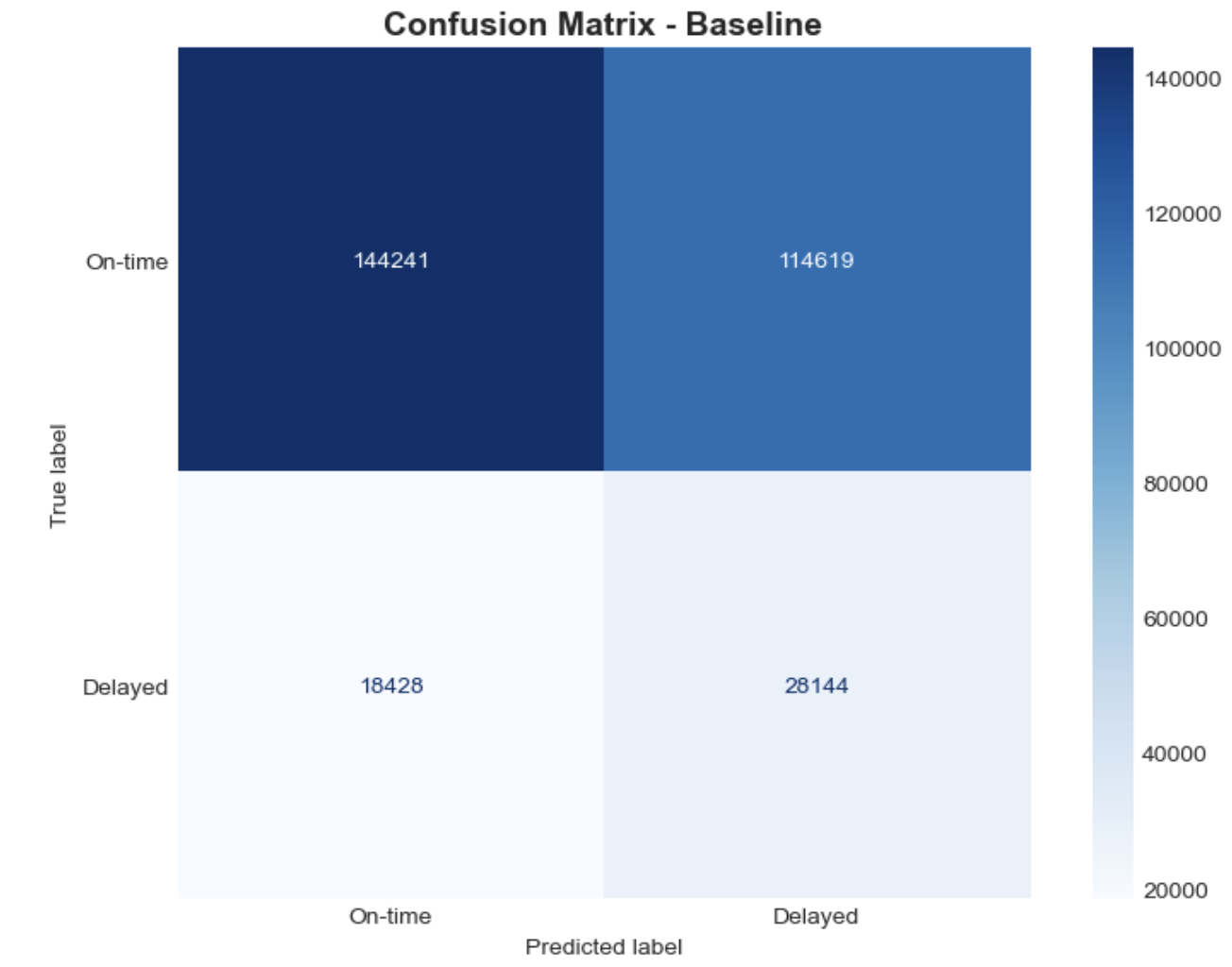
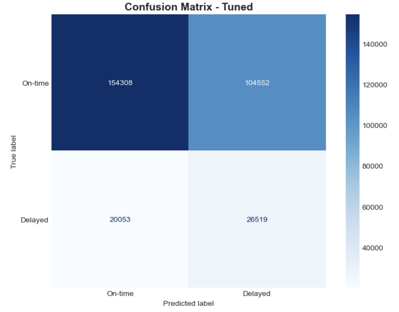
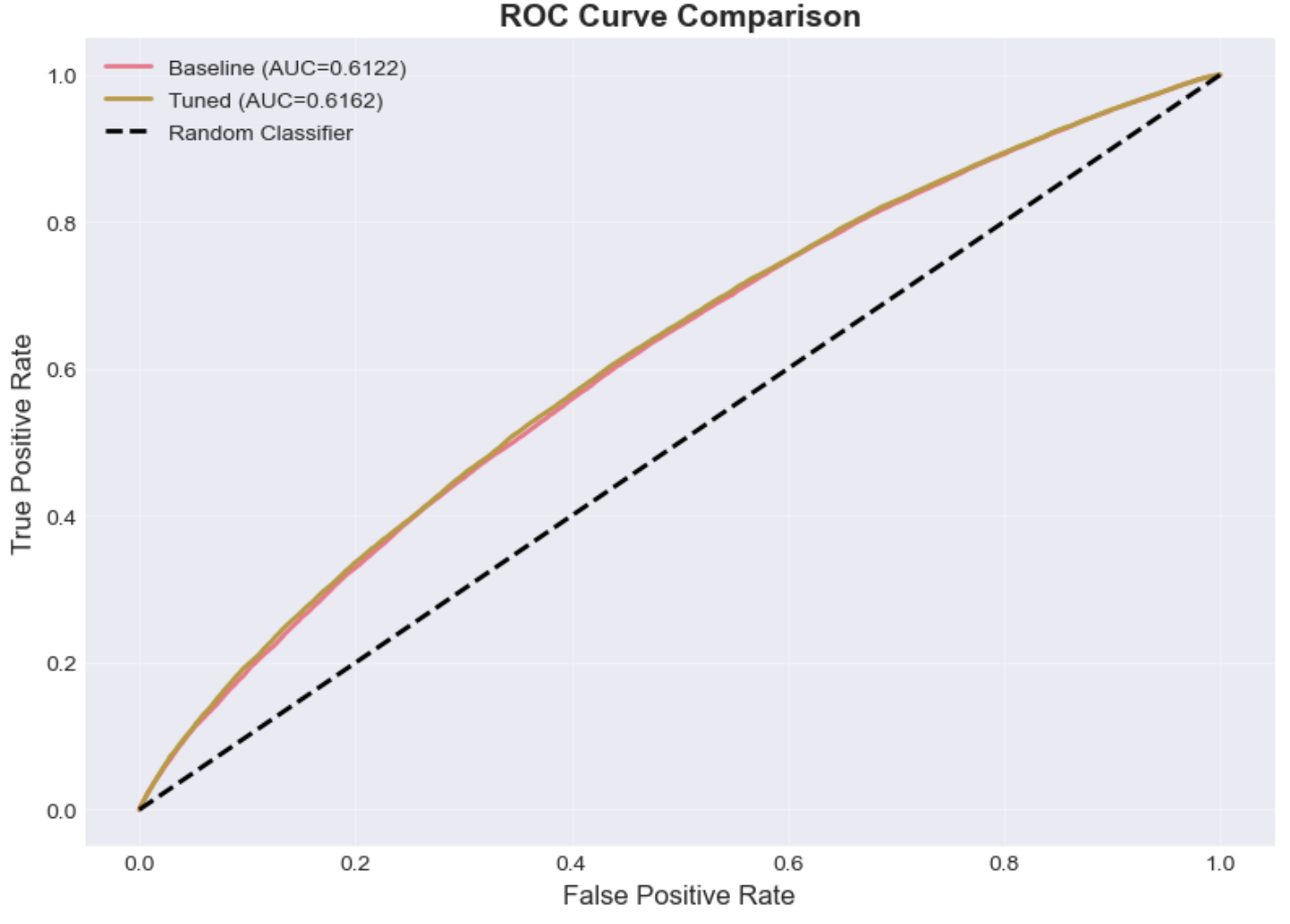
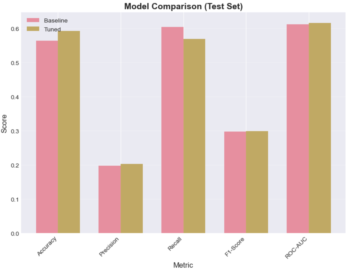
MLP Classifier
The MLP Classifier was trained to perform binary classification (the probability that a flight is delayed). We first tried implementing a baseline model, and then we conducted hyperparameter tuning via grid search and cross-validation to find optimal values for the hyperparameters. The model's performance was evaluated using Accuracy, Precision, Recall, F1-Score and ROC-AUC. The visualizations below summarize the tuned model’s ability to better classify delayed and on-time flights than the baseline.
Visualizations
Quantitative Metrics
Tuned MLP Classifier Performance
| Dataset | Accuracy | Precision | Recall | F1-Score |
|---|---|---|---|---|
| Training Set | 0.5926 | 0.2036 | 0.5739 | 0.3005 |
| Test Set | 0.5920 | 0.2023 | 0.5694 | 0.2986 |
Overfitting Analysis
| Metric | Value |
|---|---|
| Accuracy difference (train − test) | 0.0006 |
| F1 difference (train − test) | 0.0020 |
| Status | Good generalization ✓ |
Classifier Comparison: Baseline vs Tuned
| Metric | Baseline | Tuned | Improvement |
|---|---|---|---|
| Accuracy | 0.564397 | 0.592037 | 0.027640 |
| Precision | 0.197138 | 0.202325 | 0.005188 |
| Recall | 0.604312 | 0.569419 | -0.034892 |
| F1-Score | 0.297293 | 0.298565 | 0.001272 |
| ROC-AUC | 0.612242 | 0.616197 | 0.003955 |
Analysis of MLP Classifier
The tuned model shows improvements in most metrics, but the gains are small.
- The accuracy increased 2.8% (from 56.4% to 59.2%), which is the most notable improvement.
- The precision improved 0.5%: the tuned model makes marginally fewer FP predictions. However, at the expense of recall which decreased./li>
- Recall actually decreased 3.5%: the tuned model is missing more TPs than the baseline.
We observe that the tuning made the model miss more TP but it also commits less FP. This trade-off is not necessarily bad, it is reasonable that predicting that a flight will be delayed when it is not (FP) be more costly than predicting that it will not be delayed when it actually is (FN).
Also note that the tuning could have come up with a different optimal solution had we tried with more combinations. Moreover, our baseline was randomly picked, that means that we may have picked a baseline that wasn’t the “worst”, thus no “notable” improvements are seen.
Overall, the fact thet our MLP classifier's accuracy is 60% may be attributed to different factors. Firtly, due to our original dataset's quality, despite our feature engineering efforts where we take into account factors like whether it's a weekend day. Secondly, the fact that we were running locally with limited computational power limited our hyperparameter tunning. Ideally, we should try more hyperparameter combinations (hidden layer sizes, activation function, alpha, learning rate).
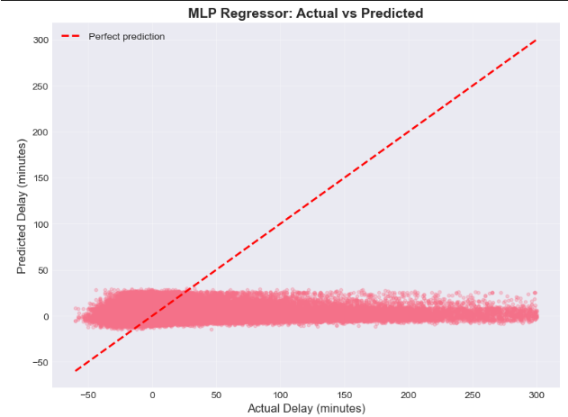
MLP Regressor
The MLP Regressor was trained to estimate the magnitude of arrival delay (in minutes), using an initial baseline configuration followed by a tuned model obtained via grid search and cross-validation. Model performance was evaluated using RMSE, MAE, and R². The results and visualizations below summarize the models’ predictive behavior and the improvements over the baseline.
Visualizations
Quantitative Metrics
Tuned MLP Performance
| Dataset | MSE | RMSE (minutes) | MAE (minutes) | R² |
|---|---|---|---|---|
| Training Set | 1175.7808 | 34.2897 | 19.7112 | 0.0260 |
| Test Set | 1181.3991 | 34.3715 | 19.8030 | 0.0247 |
Overfitting Analysis
| Metric | Value |
|---|---|
| RMSE difference (train − test) | -0.0818 |
| R² difference (train − test) | 0.0013 |
| Status | Good generalization ✓ |
Regressor Comparison: Baseline vs Tuned
| Metric | Baseline | Tuned | Improvement |
|---|---|---|---|
| RMSE (Test) | 34.4191 | 34.3715 | -0.0477 |
| MAE (Test) | 19.6952 | 19.8030 | 0.1078 |
| R² (Test) | 0.021952 | 0.024659 | 0.002706 |
| RMSE (Train) | 34.3540 | 34.2897 | -0.0644 |
| R² (Train) | 0.022301 | 0.025962 | 0.003661 |
Analysis of MLP Regressor
The tuned MLP regressor shows very similar performance on the training and test sets (RMSE ≈ 34.3 vs. 34.4 minutes, MAE ≈ 19.7 vs. 19.8 minutes, and R² ≈ 0.026 vs. 0.025), indicating good generalization and no clear signs of overfitting. However, the relatively low R² values mean that the model explains only a small portion of the variance in arrival delays.
The Actual vs Predicted plot shows that the MLP produces conservative delay estimates: predictions lie in a narrow band around small positive delays, while actual delays can be much larger (both early and late). This suggests that the model captures the general tendency of flights to have modest delays but tends to under-estimate rare, extreme disruptions.
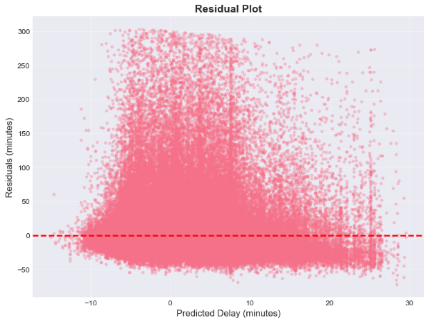
The residual plot is roughly centered around zero with no strong systematic pattern, indicating no major bias across the range of predicted delays. Nonetheless, the increasing spread and vertical “fan” of residuals for some predictions reveals that the MLP struggles to fully capture infrequent, high-impact delay events, mirroring the behavior observed for the Random Forest Regressor.
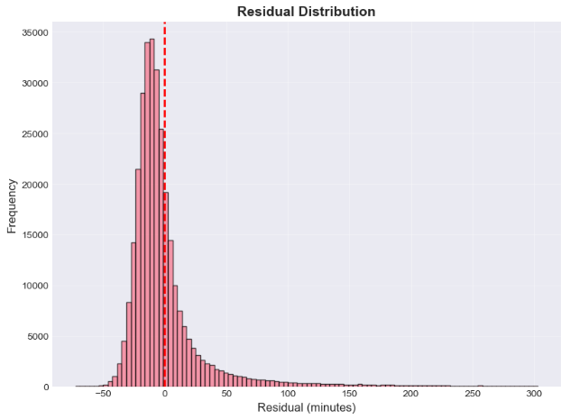
The residual distribution has a clear peak near zero and a right-skewed tail: most errors are relatively small, but there are occasional larger under-predictions when severe delays occur. This pattern is consistent with heavy-tailed delay behavior and indicates that the model is more reliable for day-to-day operations than for extreme disruptions.
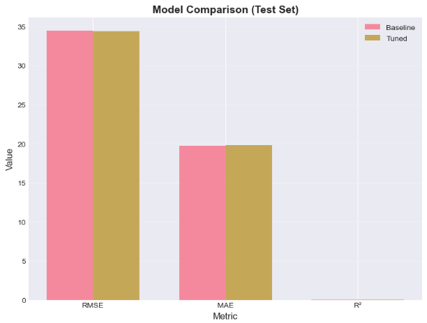
Hyperparameter tuning (two hidden layers, tanh activation, stronger regularization,
and early stopping) yields small yet consistent gains over the baseline MLP in terms of RMSE and
R², without introducing overfitting. The comparison bar plot shows that baseline and tuned
metrics are almost indistinguishable, suggesting that the original configuration was already
close to the best achievable performance with the available features.
Overall, the tuned MLP regressor exhibits behavior very similar to the Random Forest model: it generalizes well, avoids overfitting, and captures typical operations, but its predictions remain conservative and it struggles with rare, extreme delay events. As discussed for the Random Forest Regressor, these limitations arise mainly from the feature set—based solely on schedule information—rather than from the specific algorithm. Incorporating external data such as weather, airport load, or upstream rotations, or reframing the problem into delay buckets or probabilistic delay ranges, would likely enhance the practical usefulness of the MLP regressor.
XGBoost (Gradient Boosting)
XGBoost was evaluated on both the regression and classification tasks using tuned hyperparameters obtained through randomized search with 3-fold cross-validation. The model's performance was assessed using standard metrics for each task, and the results are summarized below.
Visualization
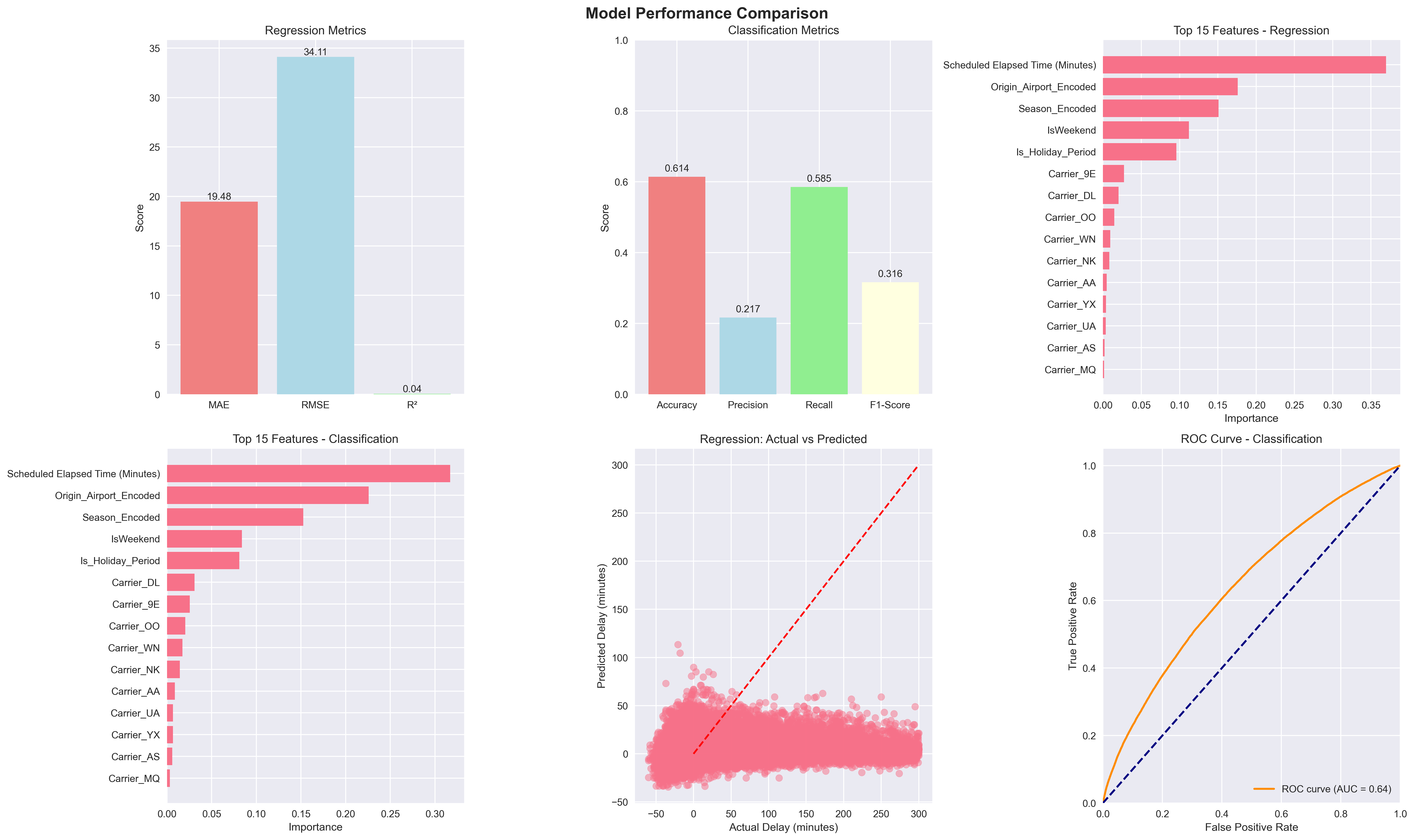
XGBoost performance summary showing regression and classification metrics.
Quantitative Metrics
Regression Model (Test Set)
| Metric | Value |
|---|---|
| MAE (Mean Absolute Error) | 19.48 minutes |
| RMSE (Root Mean Squared Error) | 34.11 minutes |
| R² (Coefficient of Determination) | 0.0392 |
| Predictions within 15 minutes | 57.1% |
Classification Model (Test Set)
| Metric | Value |
|---|---|
| Accuracy | 0.6142 |
| Precision | 0.2167 |
| Recall | 0.5851 |
| F1-Score | 0.3162 |
| ROC-AUC | 0.6430 |
Analysis of XGBoost Models
The XGBoost Regressor achieved an MAE of 19.48 minutes and an RMSE of 34.11 minutes, placing it among the best-performing models for delay magnitude prediction. However, the low R² value (0.0392) indicates that only about 4% of the variance in arrival delays is explained by the model, consistent with the limitations observed in Random Forest and MLP regressors. The fact that 57.1% of predictions fall within 15 minutes of the actual delay suggests the model provides useful estimates for typical operations, but struggles with extreme delay events.
For the XGBoost Classifier, the model achieved an accuracy of 0.6142 and an F1-score of 0.3162, with recall at 0.5851 and precision at 0.2167. These results reflect a balance between identifying delayed flights (high recall) and avoiding false alarms (lower precision). The ROC-AUC of 0.6430 indicates moderate discriminative ability, similar to Random Forest and MLP classifiers.
XGBoost's sequential boosting strategy and built-in regularization help it generalize well on structured data, but the limited feature set (lacking weather, upstream congestion, and real-time operational data) constrains its predictive power. The model performs comparably to Random Forest and MLP models, suggesting that the current bottleneck is not model capacity but rather the absence of critical external variables known to drive flight delays.
Overall, XGBoost demonstrates competitive performance and efficient training, making it a strong candidate for delay prediction systems. Future improvements could leverage its ability to incorporate external features such as weather forecasts, air traffic load, and upstream delay propagation, which are expected to significantly enhance both regression and classification performance.
Conclusion and Model Comparison
In this project, we evaluated multiple machine learning models for both classification (predicting whether a flight will be delayed) and regression (predicting the delay magnitude in minutes). Below we summarize the performance of each model category.
Summary of Classification Models
| Model | Accuracy | Precision | Recall | F1-Score | ROC–AUC | Key Insight |
|---|---|---|---|---|---|---|
| Logistic Regression (Balanced) | 0.600 | 0.186 | 0.483 | 0.268 | 0.580 | Linear baseline; struggles with nonlinear patterns. |
| Random Forest Classifier (Balanced) | 0.633 | 0.218 | 0.550 | 0.313 | 0.637 | Best recall; robust to imbalance. |
| MLP Classifier (Tuned) | 0.592 | 0.202 | 0.569 | 0.299 | 0.616 | Comparable to RF; limited improvement. |
| XGBoost Classifier | 0.614 | 0.217 | 0.585 | 0.316 | 0.643 | Best ROC–AUC; strong boosting performance. |
Summary of Regression Models
| Model | RMSE (min) | MAE (min) | R² | Key Insight |
|---|---|---|---|---|
| Random Forest Regressor | 34.17 | 19.53 | 0.036 | Stable but underestimates large delays. |
| MLP Regressor (Tuned) | 34.37 | 19.80 | 0.025 | Smooth predictions, similar limitations as RF. |
| XGBoost Regressor | 34.11 | 19.48 | 0.039 | Best regression performance, still low variance explained. |
Overall, tree ensembles (Random Forest, XGBoost) consistently outperformed linear and neural models in both classification and regression tasks, confirming the importance of nonlinear interactions in flight delay prediction. Classification models achieved moderate success, particularly XGBoost and Random Forest, highlighting that delay detection is feasible from schedule-based features alone.
Regression models, however, struggled to explain variance in delay magnitude, with all R² scores below 0.04. This limitation reflects the absence of external factors such as weather, airport congestion, and upstream delay propagation, which are essential for accurate delay forecasting.
Future improvements should incorporate richer datasets and consider probabilistic delay ranges or multi-class delay buckets rather than exact delay values, enabling more actionable and reliable predictions for real-world operations.
References
[1] I. Hatipoğlu and Ö Tosun, “Predictive modeling of flight delays at an airport using machine learning methods,” Applied Sciences, vol. 14, no. 13, p. 5472, 2024.
[2] N. Kuhn and N. Jamadagni, Application of machine learning algorithms to predict flight arrival delays. Course Project Report CS229, Stanford University, 2024. [Online]. Available: https://cs229.stanford.edu/proj2017/final-reports/5243248.pdf
[3] P. Meel, M. Singhal, M. Tanwar and N. Saini, "Predicting flight delays with error calculation using machine learned classifiers," 7th International Conference on Signal Processing and Integrated Networks (SPIN)*, 2020, pp. 71-76.
[4] J. Li et al., "Prediction of flight arrival delay time using U.S. Bureau of Transportation Statistics," 2023 IEEE Symposium Series on Computational Intelligence (SSCI), Mexico, 2 023, pp. 603-608.
[5] T. K. Huynh, T. Cheung and C. Chua, "A systematic review of flight delay forecasting models," 2024 7th International Conference on Green Technology and Sustainable Development (GTSD), 2024, pp. 533-540.
[6] Bureau of Transportation Statistics, U.S. Department of Transportation, 2025. “On-Time Performance Data (Arrivals),” distributed by Bureau of Transportation Statistics. Available: https://www.transtats.bts.gov/ONTIME/Arrivals.aspx
[7] Bureau of Transportation Statistics, U.S. Department of Transportation, 2024. “Number of Delayed Flights in 2024,” distributed by Bureau of Transportation Statistics. Available: https://www.transtats.bts.gov/Marketing_Annual.aspx?heY_fryrp6lrn4=FDFI&heY_fryrp6Z106u=J&heY_gvzr=E&heY_fryrp6v10=E
[8] Federal Aviation Administration, 2020, "Cost of Delay Estimates," distributed by Federal Aviation Administration (FAA).
[9] R. G, K. Vijaya, S. Sadesh, A. P. M, M. P. V and M. S. Kumar, "Predicting Flight Delays and Error Calculation Using Machine Learning Classifiers," 5th International Conference on Electronics and Sustainable Communication Systems (ICESC), India, 2024, pp. 1238-1244.